Blob analysis with OpenCV in Python

Here’s my methodology for performing a blob analysis from binary images in OpenCV using Python code.

A blob is a binary large object. The purpose of blob extraction is to isolate the blobs (or objects) in a binary image. A blob consists of a group of connected pixels. Whether or not two pixels are connected is defined by the connectivity, that is, which pixels are neighbours and which are not.

Blob analysis is a useful and commonplace tool in image analysis to assist in the identification and measurement of features in an image. In a typical scenario, a RGB image would be converted to greyscale, then thresholded and binarised before a blob analysis is completed.

Methods for blob analysis exist in many languages and platforms but there isn’t a simple procedure or process when using OpenCV in Python. For this reason, I have documented my approach to the problem in terms that I hope will make sense and be easy to implement.

Packages and Setup

For this example, I am using OpenCV 3.4.13.47 under Python 3.7.4 with the following packages:

• MatPlotLib
• OpenCV (cv2)
• NumPy
• CSV

These are loaded as follows:

import matplotlib as mpl
import matplotlib.pyplot as plt
import cv2
import numpy as np
import csv

I will be displaying blobs with different colours, so I need a list of RGB colours to draw upon. This will do:

colours = [(230, 63, 7), (48, 18, 59), (68, 81, 191), (69, 138, 252), (37, 192, 231), (31, 233, 175), (101, 253, 105), (175, 250, 55), (227, 219, 56), (253, 172, 52), (246, 108, 25), (216, 55, 6), (164, 19, 1), (90, 66, 98), (105, 116, 203), (106, 161, 253), (81, 205, 236), (76, 237, 191), (132, 253, 135), (191, 251, 95), (233, 226, 96), (254, 189, 93), (248, 137, 71), (224, 95, 56), (182, 66, 52), (230, 63, 7), (48, 18, 59), (68, 81, 191), (69, 138, 252), (37, 192, 231), (31, 233, 175), (101, 253, 105), (175, 250, 55), (227, 219, 56), (253, 172, 52), (246, 108, 25), (216, 55, 6), (164, 19, 1), (90, 66, 98), (105, 116, 203), (106, 161, 253), (81, 205, 236), (76, 237, 191), (132, 253, 135), (191, 251, 95), (233, 226, 96), (254, 189, 93), (248, 137, 71), (224, 95, 56), (182, 66, 52)]

Preparing an Image

The image that I intend performing a blob analysis on is the below map of Australia, with the various states and territories demarcated.

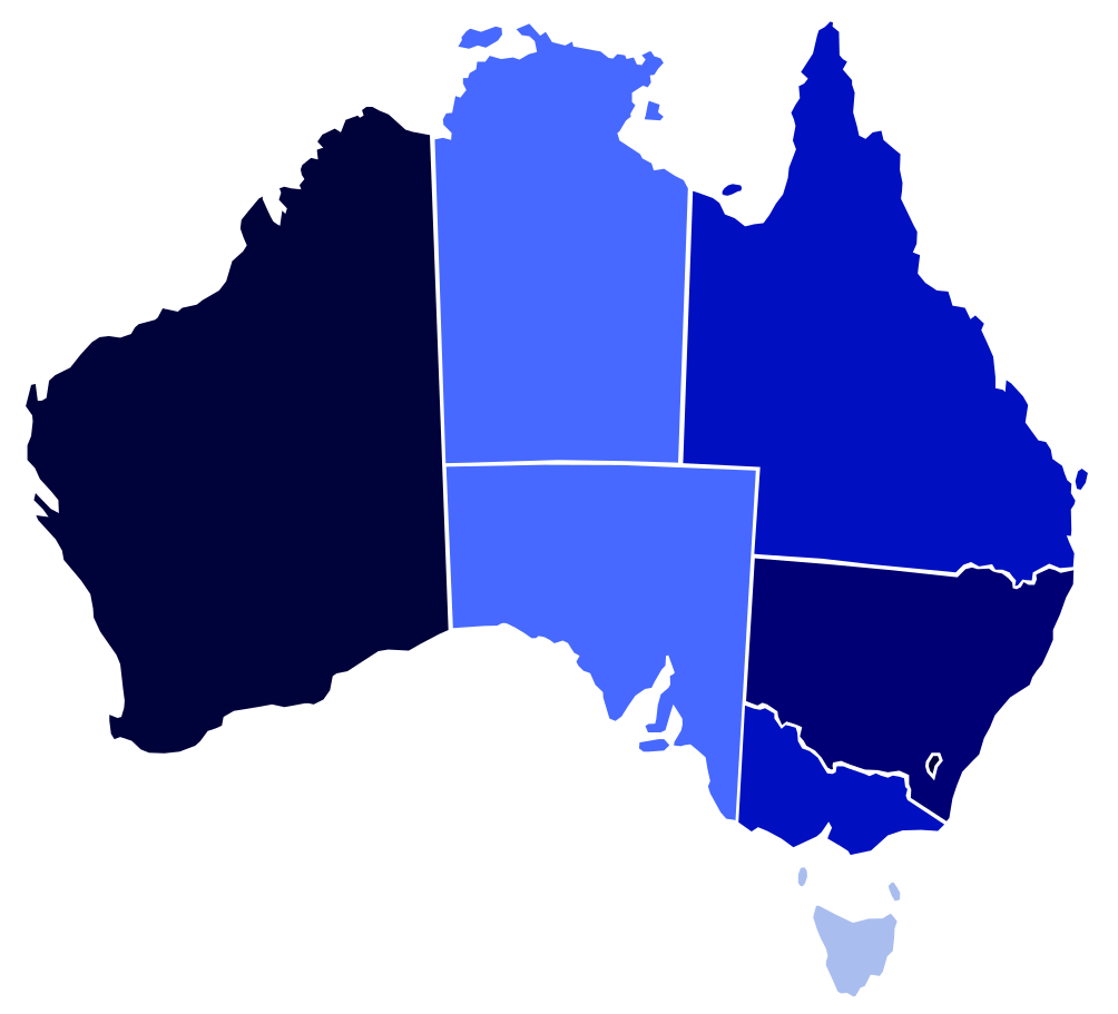
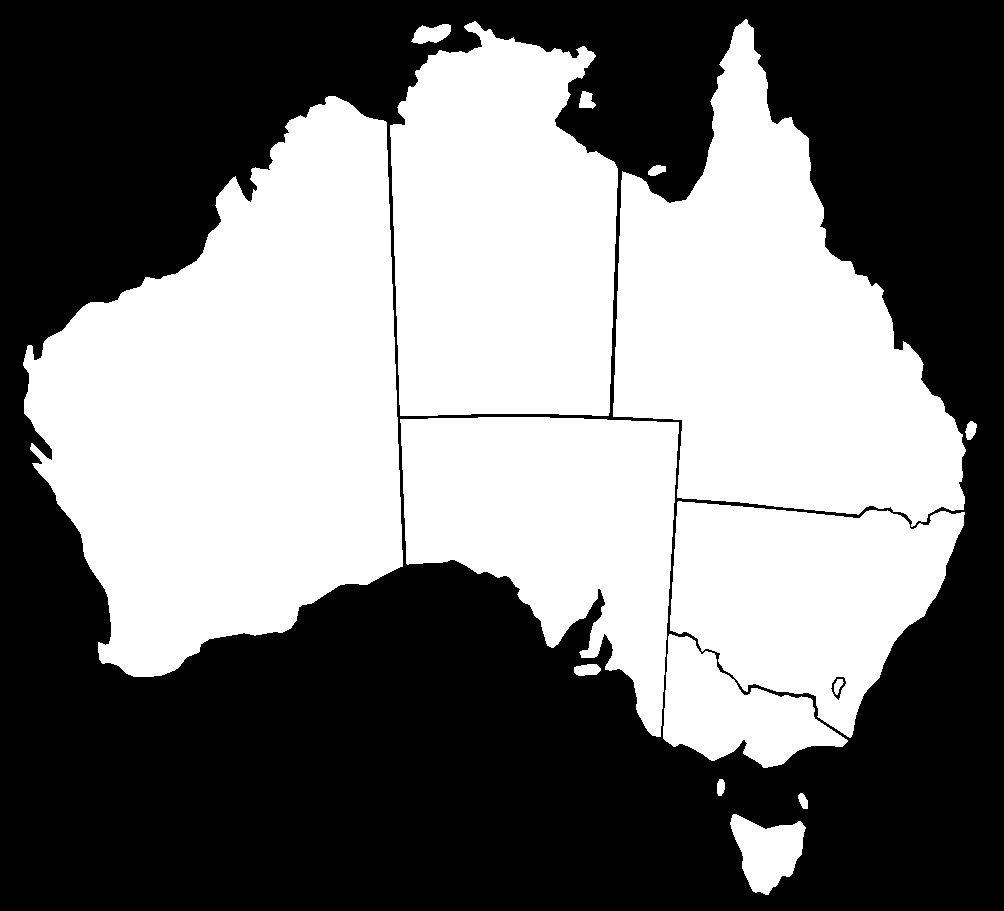
The image will be loaded, converted to greyscale, inverted, and then binarised with a threshold as follows:

img = cv2.imread('/path/to/australian_states.png') #Read image
grey = cv2.cvtColor(img, cv2.COLOR_BGR2GRAY) # Convert to greyscale
grey_inv = cv2.bitwise_not(grey) #Inverse
ret,thresh_au = cv2.threshold(grey_inv,20,255,cv2.THRESH_BINARY) #Threshold

Here is the result:

Blob Analysis

First, we need to find the contours in the image, which is fairly simple:

contours = cv2.findContours(thresh_au, cv2.RETR_EXTERNAL, cv2.CHAIN_APPROX_SIMPLE)
contours = contours[0] if len(contours) == 2 else contours[1]

The next process is a bit more complex, but its purpose is to perform a series of calculations on each of the blobs in the image so that they can be reported later-on. These are wrapped in a function which I have called blob_properties:

def blob_properties(contours):
  cont_props= []
  i = 0
  for cnt in contours:
    area= cv2.contourArea(cnt)
    perimeter = cv2.arcLength(cnt,True)
    convexity = cv2.isContourConvex(cnt)
    x1,y1,w,h = cv2.boundingRect(cnt)
    x2 = x1+w
    y2 = y1+h
    aspect_ratio = float(w)/h
    rect_area = w*h
    extent = float(area)/rect_area
    hull = cv2.convexHull(cnt)
    hull_area = cv2.contourArea(hull)
    solidity = float(area)/hull_area
    (xa,ya),(MA,ma),angle = cv2.fitEllipse(cnt)
    rect = cv2.minAreaRect(cnt)
    (xc,yc),radius = cv2.minEnclosingCircle(cnt)
    ellipse = cv2.fitEllipse(cnt)
    rows,cols = img.shape[:2]
    [vx,vy,xf,yf] = cv2.fitLine(cnt, cv2.DIST_L2,0,0.01,0.01)
    lefty = int((-xf*vy/vx) + yf)
    righty = int(((cols-xf)*vy/vx)+yf)
    # Add parameters to list
    add = i+1, area, round(perimeter, 1), convexity, round(aspect_ratio, 3), round(extent, 3), w, h, round(hull_area, 1), round(angle, 1), x1, y1, x2, y2,round(radius, 6), xa, ya, xc, yc, xf[0], yf[0], rect, ellipse, vx[0], vy[0], lefty, righty
    cont_props.append(add)
    i += 1

  return cont_props

Some of these are directly informative and some of them will help with derived calculations later-on. They key measures that I want to return for each blob are:

• Area
• Perimeter
• Convexity
• Convex hull area
• Aspect ratio
• Extent
• Width
• Height
• Fitted ellipse area
• Fitted ellipse radius
• Straight bounding rectangle (x₁, y₁, x₂, y₂)

For the biggest blob, I’d like to plot:

• Straight bounding rectangle
• Rotated rectangle
• Minimum enclosing circle
• Fitted ellipse
• Fitted line angle

The next step towards this is to sort my contours by the contour area from largest to smallest:

sorted_contours= sorted(contours, key=cv2.contourArea, reverse= True)

The result of this function are the aforementioned properties contained in a Python list. We’ll come back to that.

Let’s grab that data and prepare to plot it:

blobs_data = blob_properties(sorted_contours)
image_plot = img.copy()

I can use a For loop to iterate over the sorted list of contour and blob data and label each one on an image. This references the colours list at the top of this article.

for rows in blobs_data:
  pos = blobs_data[i]
  inverted_colours = (255-colours[i][0],255-colours[i][1],255-colours[i][2])
  cv2.drawContours(image_plot, [sorted_contours[i]], -1, colours[i], -1) #, colours[i], thickness=cv2.FILLED)
  cv2.putText(image_plot, str(pos[0]), (int(pos[19]), int(pos[20])), cv2.FONT_HERSHEY_SIMPLEX, 1, inverted_colours, 2, cv2.LINE_AA)
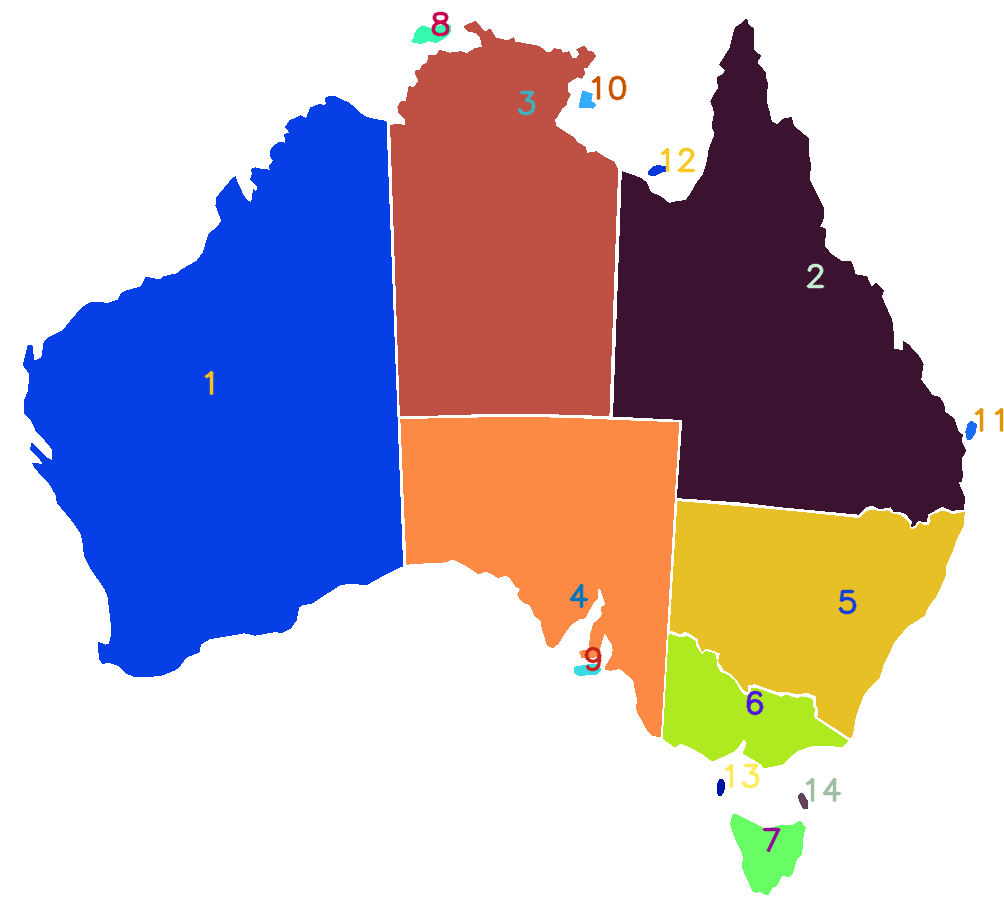
  i += 1

For clarity, I have not only colour-coded each blob, but I have also appended a label so that I can relate it back to the data. To do this, I have used the inverse colour of the blob so that the text remains legible: this is done by calculating the sum of 255-R, 255-G and 255-B.

Here is the result:

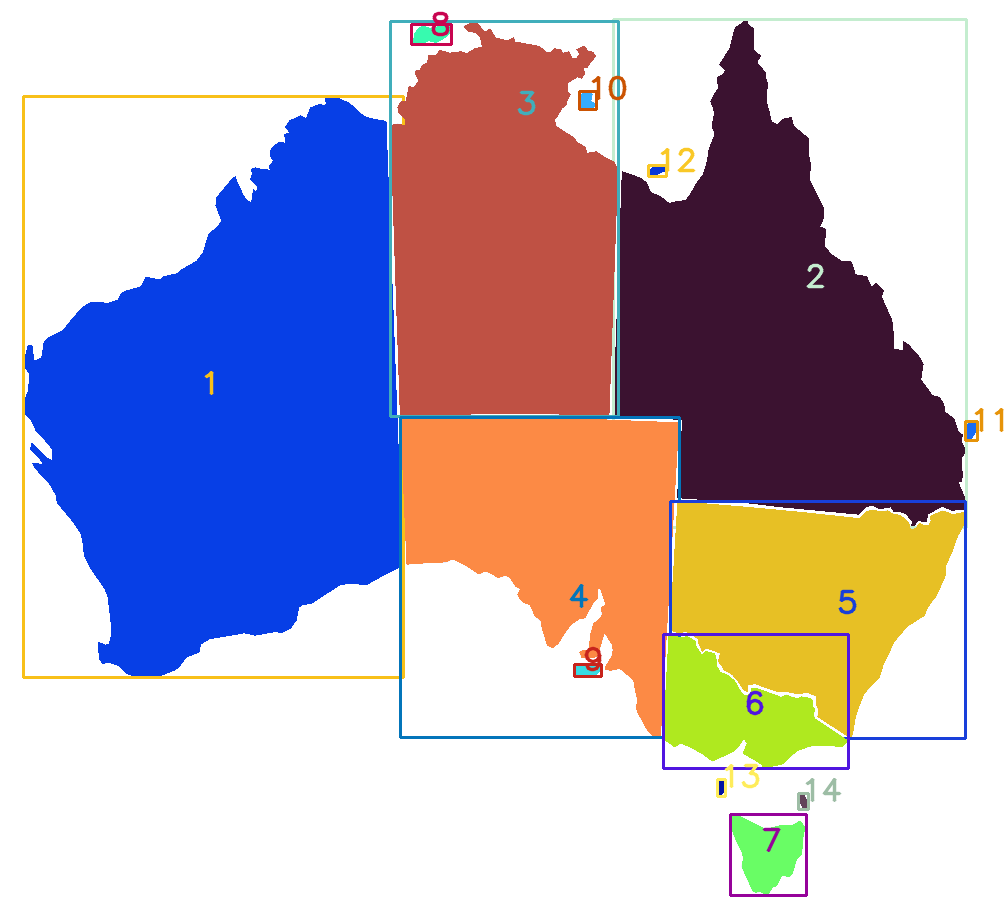
I could add more data to this graphic, depending on the application. For instance, if I wanted to show the bounding rectangles, I could add the following line:

cv2.rectangle(image_plot, (pos[10], pos[11]), (pos[12], pos[13]), inverted_colours, 2)

Here is the result, but it’s getting messy:

The data for each blob can then be collected into a CSV for review:

header = ['blob_id','area','perimeter','convexity','aspect_ratio','extent','width','height','hull_area','ellipse_angle','rect_x1','rect_y1','rect_x2','rect_y2','radius','xa','ya','xc','yc','xf','yf','min_area_rectangle','ellipse','vx','vy','left_y','right_y']

with open("/path/to/australian_states.csv", 'w', newline='') as file:
  dw = csv.DictWriter(file, delimiter=',', fieldnames=header)
  dw.writeheader()
  writer = csv.writer(file)
  writer.writerows(blobs_data)

The final result is a CSV containing blob data and an image showing the identification of each. Of course this example could be applied to all manner of applications.

Further analysis

Let’s say that you wanted to identify and then plot the details of the biggest blob in the image (in our case, the State of Western Australia).

To plot the rotated rectangle and minimum enclosing circle, we need to perform a few more calculations:

# Rotated rectangle
rect = blobs_data[0][21]
box = cv2.boxPoints(rect)
box = np.int0(box)

# Mimimum enclosing circle
centre = (int(blobs_data[0][17]),int(blobs_data[0][18]))
radius = int(blobs_data[0][14])

Plotting then becomes fairly straightforward:

image_plot2 = img.copy()

pos = blobs_data[0]
rows,cols = img.shape[:2]
cv2.rectangle(image_plot2, (pos[10], pos[11]), (pos[12], pos[13]), colours[1], 2) # Bounding rectangle
cv2.drawContours(image_plot2,[box],0,colours[4],2) # Rotated rectangle
cv2.circle(image_plot2,centre,radius,colours[7],2) # Minimum Enclosing Circle
cv2.ellipse(image_plot2,pos[22],colours[10],2) # Fitted ellipse
cv2.line(image_plot2,(cols-1,pos[26]),(0,pos[25]),colours[19],2) # Fitted line

The result is this:

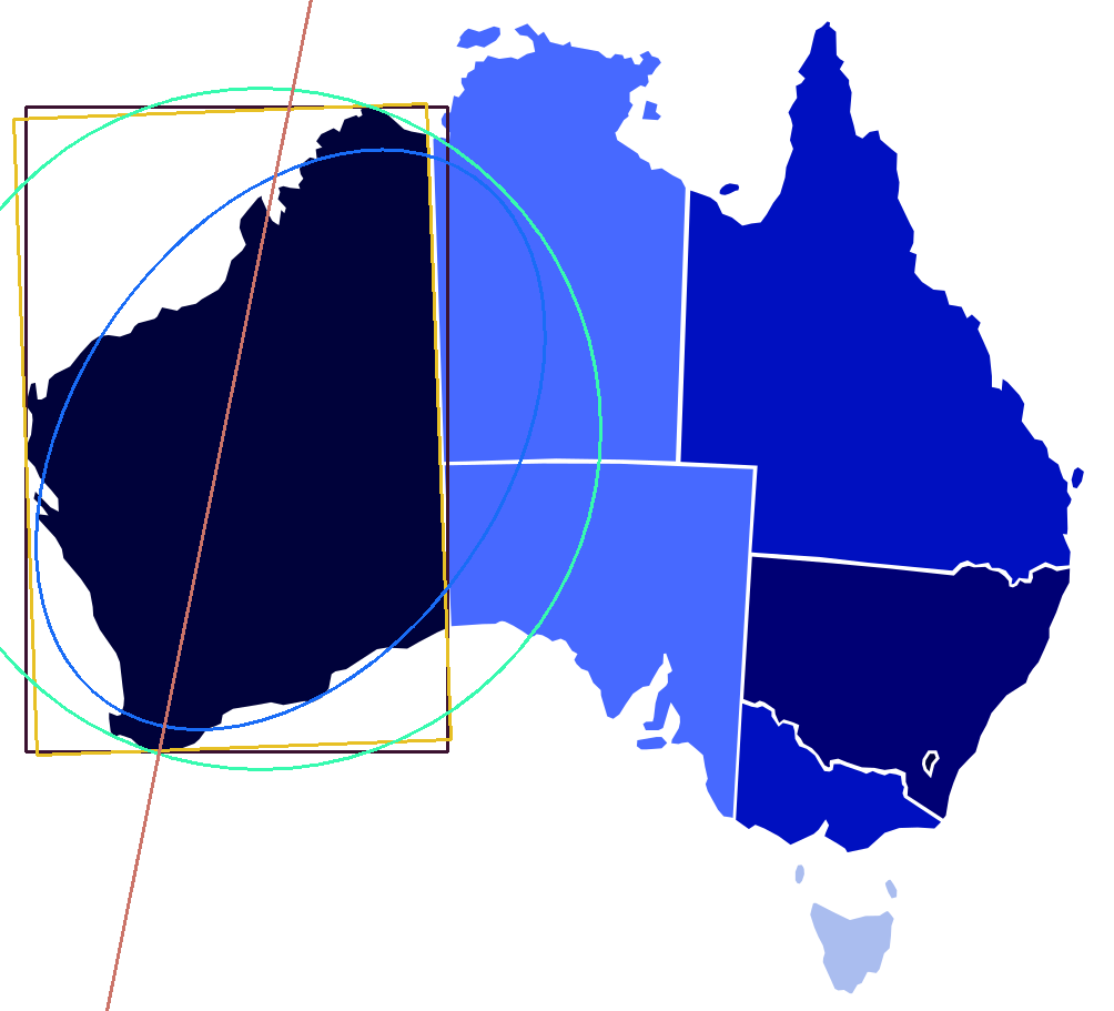
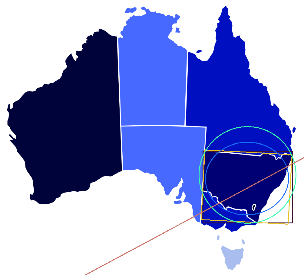
Owing to the size of the blob and its position relative to the size of the image, some of the details are cropped. It is not too difficult to adjust the code and focus on a different blog such as New South Wales (number 5):

What we have ended-up with is a complete blob analysis that counts the number of objects in the image and measures them with a variety of matrices.

The full code for this example is available on GitHub Gist.

Have Your Say

Δ